Portfolio 3
The projects should be numbered consecutively (i.e., in the order in which you began them), and should include for each project a description of the goal, the product (computer program, hand graph, computer graph, etc.), the data, and some interpretation. Reports must be reproducible and of high quality in terms of writing, grammar, presentation, etc.
The primary aim of this portfolio is to generate a distribution of sample correlation coefficients, given a certain n and population correlation. A secondary aim is to generate a plot of this distribution that I can share with my class.
I’m starting by generating sample correlations themselves (rather than the data sets). I’m going to assume normality. Although this assumption is not fully accurate (esp. for larger correlations), it should be reasonably close. It will thus help serve as a “reality check” to ensure that my next approach is operating correctly.
Note: Gnambs (2023) recommends the following formula for the standard deviation: (1-r2) / sqr (n-3)
Load packages and data
if (!require("ggplot2")) install.packages("ggplot2")
library(ggplot2)
if (!require("MASS")) install.packages("MASS")
library(MASS)
if (!require("tidyverse")) install.packages("tidyverse")
library(tidyverse)set.seed(123)For this example, the sd is approximately .14
corr_ds1 <- data.frame(id = 1:10000, corr = rnorm(10000, mean = .20, sd = .14))ggplot(data = corr_ds1, mapping = aes(x = corr)) +
geom_histogram() +
labs(title = "Distribution of Sample Correlations, r = .20, n = 50")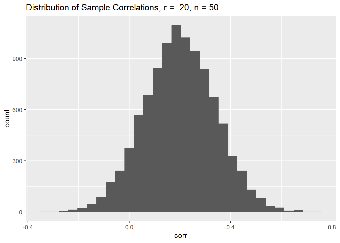
This seems to work well. Before proceeding, I’d like to calculate the percentage of sample correlations that are less than zero.
corr_ds1 <- corr_ds1 %>%
  mutate (neg_corr = case_when (
    corr < 0 ~ 1,
    corr >= 0 ~ 0 ))
perc_neg_corr <- corr_ds1 %>%
  summarize(perc_neg = mean(neg_corr))
Trying this again using a formula for sd.
corr_ds2 <- data.frame(id = 1:10000, corr = rnorm(10000, mean = .20, sd = (1-(.2)*(.2))/(sqrt(50-3)) ))corr_ds2 <- corr_ds2 %>%
mutate (neg_corr = case_when (
corr < 0 ~ 1,
corr >= 0 ~ 0 ))
perc_neg_corr2 <- corr_ds2 %>%
summarize(perc_neg = mean(neg_corr))This computes the same percentage of negative correlations, so this is working well. This will be necessary when trying to turn this into a function.
My next step is to do that – turn the above set of commands into a function.
simulate_r_practice <- function(r) {
  sample_r_practice <- rnorm(1,mean = r, sd = (1-(r)*(r))/(sqrt(50-3))  )
  return(sample_r_practice)
}
Now trying it out
simulate_r_practice(.2)## [1] 0.08289304This seems to work!
Now I’m going to create another function, which includes both r and n.
simulate_r_practice2 <- function(r,n) {
  sample_r_practice2 <- rnorm(1,mean = r, sd = (1-(r)*(r))/(sqrt(n-3))  )
  return(sample_r_practice2)
}
Now trying it out
simulate_r_practice2(.2, 50)## [1] 0.1691131This also seems to work. Yea. Next, I will try to get it to generate the full data set of 10,000 individuals.
corr_ds <- data.frame(id = 1:10000, corr = replicate (10000, simulate_r_practice2 (.2,50) ))This worked well, but I didn’t get to specify the r and n, so doesn’t really do what I want.
Now trying to create a function that creates the entire data frame.
simulate_r_dataframe <- function(r, n) {
  corr_values <- replicate(10000, simulate_r_practice2(r, n))
  simulate_r_ds <- data.frame(id = 1:10000, corr = corr_values)
  assign("simulated_data", simulate_r_ds, envir = .GlobalEnv)
}
simulate_r_dataframe(.2, 50)Okay, that finally worked. That was difficult. Now to add pop_r and n to the data file.
simulate_r_dataframe2 <- function(r, n) {
  corr_values <- replicate(10000, simulate_r_practice2(r, n))
  simulate_r_ds <- data.frame(id = 1:10000, corr = corr_values, pop_r = r, n = n)
  assign("simulated_data", simulate_r_ds, envir = .GlobalEnv)
}
simulate_r_dataframe2(.2, 50)Finally got something to work on the first try.
Now I’m going to try to make my data frame have a name that includes the values entered in the function.
simulate_r_dataframe3 <- function(r, n) {
  corr_values <- replicate(10000, simulate_r_practice2(r, n))
  simulate_r_ds <- data.frame(id = 1:10000, corr = corr_values, pop_r = r, n = n)
  df_name <- paste0("simulated_data_", r, "_", n)
  assign(df_name, simulate_r_ds, envir = .GlobalEnv)
}
simulate_r_dataframe3(.20, 50)It works.
So at this point, I have a large number of files with all sorts of weird names. I’m going to now create a new set of data files with “final” in the name that will produce the final elements of what I want.
simulate_individual_r_final <- function(r,n) {
  simulate_individual_r_final <- rnorm(1,mean = r, sd = (1-(r)*(r))/(sqrt(n-3))  )
  return(simulate_individual_r_final)
}
final_simulate_dataframe <- function(r, n) {
corr_values <- replicate(10000, simulate_individual_r_final(r, n))
simulate_r_ds <- data.frame(id = 1:10000, corr = corr_values, pop_r = r, n = n)
df_name <- paste0("final_simulated_data_", r, "_", n)
assign(df_name, simulate_r_ds, envir = .GlobalEnv)
}final_simulate_dataframe(.10, 20)
final_simulate_dataframe(.10, 50)
final_simulate_dataframe(.10, 100)
final_simulate_dataframe(.20, 20)
final_simulate_dataframe(.20, 50)
final_simulate_dataframe(.20, 100)
final_simulate_dataframe(.30, 20)
final_simulate_dataframe(.30, 50)
final_simulate_dataframe(.30, 100)
final_simulate_dataframe(.40, 20)
final_simulate_dataframe(.40, 50)
final_simulate_dataframe(.40, 100)
final_simulate_dataframe(.50, 20)
final_simulate_dataframe(.50, 50)
final_simulate_dataframe(.50, 100)now need to bind the data files .
simulated_data_final <- bind_rows(final_simulated_data_0.1_20, final_simulated_data_0.1_50, final_simulated_data_0.1_100, final_simulated_data_0.2_20, final_simulated_data_0.2_50, final_simulated_data_0.2_100, final_simulated_data_0.3_20, final_simulated_data_0.3_50, final_simulated_data_0.3_100, final_simulated_data_0.4_20, final_simulated_data_0.4_50, final_simulated_data_0.4_100, final_simulated_data_0.5_20, final_simulated_data_0.5_50, final_simulated_data_0.5_100)Adding in the number of negative corrs.
simulated_data_final <- simulated_data_final %>%
  mutate (neg_corr = case_when (
    corr < 0 ~ 1,
    corr >= 0 ~ 0 ))
perc_neg_corr_final <- simulated_data_final %>%
   group_by(pop_r, n) %>%
  summarize(perc_neg = mean(neg_corr))
Okay, so this generated what I wanted. It does require me to go in and specify the names of the data frames to bind. Ideally that shouldn’t be necessary, but this has already taken 5-6 hours so I’m going to just go with that.
So that worked well overall, but unfortunately, it’s really not the way to do this, because it’s assuming that r is normal, which it isn’t, especially for r’s far from 0. So I’m going to start over, generating values of x and y and computing r’s. Thankfully (I think…) once I can generate a data frame with r’s, I should be able to re-use the rest of my code to finish.
First need to make sure I can get the commands to work with a certain correlation.
# Define mean and covariance matrix
mean_x_y <- c(0, 0)
cov_matrix <- matrix(c(1, .20,
                       .20, 1), ncol = 2)

# Generate correlated data
x_y_data_matrix_practice <- mvrnorm(n = 10000, mu = mean_x_y, Sigma = cov_matrix, empirical = FALSE)
colnames(x_y_data_matrix_practice) <- c("x", "y")
x_y_data_practice <- as.data.frame(x_y_data_matrix_practice)
Checking:
x_y_data_practice %>%
  summarize(
    corr = cor(x, y)
            ) %>%
    return(corr)
## corr
## 1 0.2003635Okay, this worked well. It generated a correlation close to .20, and when I ran it again it was still very close to .20 but slightly different.
Next I need to turn this into a function to generate x and y, for a given r and n.
simulate_individual_x_y <- function(r,n) {
 mean_x_y <- c(0, 0)
 cov_matrix <- matrix(c(1, r,
                         r, 1), ncol = 2)
 x_y_data_matrix <- mvrnorm(n = n, mu = mean_x_y, Sigma = cov_matrix, empirical = FALSE)
 colnames(x_y_data_matrix) <- c("x", "y")
 x_y_data <- as.data.frame(x_y_data_matrix)
 df_name <- paste0("individual_x_y_", r, "_", n)
 assign(df_name, x_y_data, envir = .GlobalEnv)
} simulate_individual_x_y(.20,1000)individual_x_y_0.2_1000 %>%
summarize(
corr = cor(x, y)
) %>%
return(corr)## corr
## 1 0.1888047Okay, I tried this a bunch of times and got different correlations. They were all close to .20, but not as close as when I used n of 10,000. So this is working well.
Unfortunately, that function just creates one correlation. I need a function that does this 10,000 times.
I spent a while trying to do that, but I think I need to have it create the correlation as part of the function. I’m going to revise the function now.
final_simulate_individual_x_y <- function(r,n) {
 mean_x_y <- c(0, 0)
 cov_matrix <- matrix(c(1, r,
                         r, 1), ncol = 2)
 x_y_data_matrix <- mvrnorm(n = n, mu = mean_x_y, Sigma = cov_matrix, empirical = FALSE)
 colnames(x_y_data_matrix) <- c("x", "y")
 x_y_data <- as.data.frame(x_y_data_matrix)
 df_name <- paste0("individual_x_y_", r, "_", n)
 assign(df_name, x_y_data, envir = .GlobalEnv)
 calculated_corr <- cor(x_y_data$x, x_y_data$y)
 return(calculated_corr)
} final_simulate_individual_x_y(.20,1000)## [1] 0.2287051simulate_repeated_x_y <- function(r, n) {
correlations <- replicate(10000, final_simulate_individual_x_y (r, n))
correlation_results <- data.frame(id = 1:100, corr = correlations, pop_r = r, n = n)
df_name <- paste0("simulated_r_from_xy", r, "_", n)
assign(df_name, correlation_results, envir = .GlobalEnv)
}simulate_repeated_x_y(.20,50)Okay, I’m now at the point where I was at when I just simulated the code directly, so I’ll use the same logic as before and just change the file names.
simulate_repeated_x_y(.10, 20)
simulate_repeated_x_y(.10, 50)
simulate_repeated_x_y(.10, 100)
simulate_repeated_x_y(.20, 20)
simulate_repeated_x_y(.20, 50)
simulate_repeated_x_y(.20, 100)
simulate_repeated_x_y(.30, 20)
simulate_repeated_x_y(.30, 50)
simulate_repeated_x_y(.30, 100)
simulate_repeated_x_y(.40, 20)
simulate_repeated_x_y(.40, 50)
simulate_repeated_x_y(.40, 100)
simulate_repeated_x_y(.50, 20)
simulate_repeated_x_y(.50, 50)
simulate_repeated_x_y(.50, 100)
now need to bind the data files .
simulated_data_final_xy <- bind_rows(simulated_r_from_xy0.1_20, simulated_r_from_xy0.1_50, simulated_r_from_xy0.1_100, simulated_r_from_xy0.2_20, simulated_r_from_xy0.2_50, simulated_r_from_xy0.2_100, simulated_r_from_xy0.3_20, simulated_r_from_xy0.3_50, simulated_r_from_xy0.3_100, simulated_r_from_xy0.4_20, simulated_r_from_xy0.4_50, simulated_r_from_xy0.4_100, simulated_r_from_xy0.5_20, simulated_r_from_xy0.5_50, simulated_r_from_xy0.5_100)Adding in the number of negative corrs.
simulated_data_final_xy <- simulated_data_final_xy %>%
  mutate (neg_corr_xy = case_when (
    corr < 0 ~ 1,
    corr >= 0 ~ 0 ))
perc_neg_corr_final_xy <- simulated_data_final_xy %>%
   group_by(pop_r, n) %>%
  summarize(perc_neg_xy = mean(neg_corr_xy))
Yea, this worked!! And the results are very similar to the ones when I simulated r directly, so that’s good reliability. I’m not sure to what extent the differences are due to chance or the more accurate approach in the later case, so I’ll use the latter approach.
The last thing is to make some graphs. I’m going to make two types.
One is to make histograms. I’ll do this for just the correlations of .20
simulated_data_final_xy_.20 <- bind_rows(simulated_r_from_xy0.2_20, simulated_r_from_xy0.2_50, simulated_r_from_xy0.2_100)ggplot(data = simulated_data_final_xy_.20, mapping = aes(x = corr)) +
geom_histogram() +
facet_grid (~ n) +
labs(title = "Distribution of Sample Correlations, r = .20") +
scale_y_continuous(name = "Count", breaks = NULL)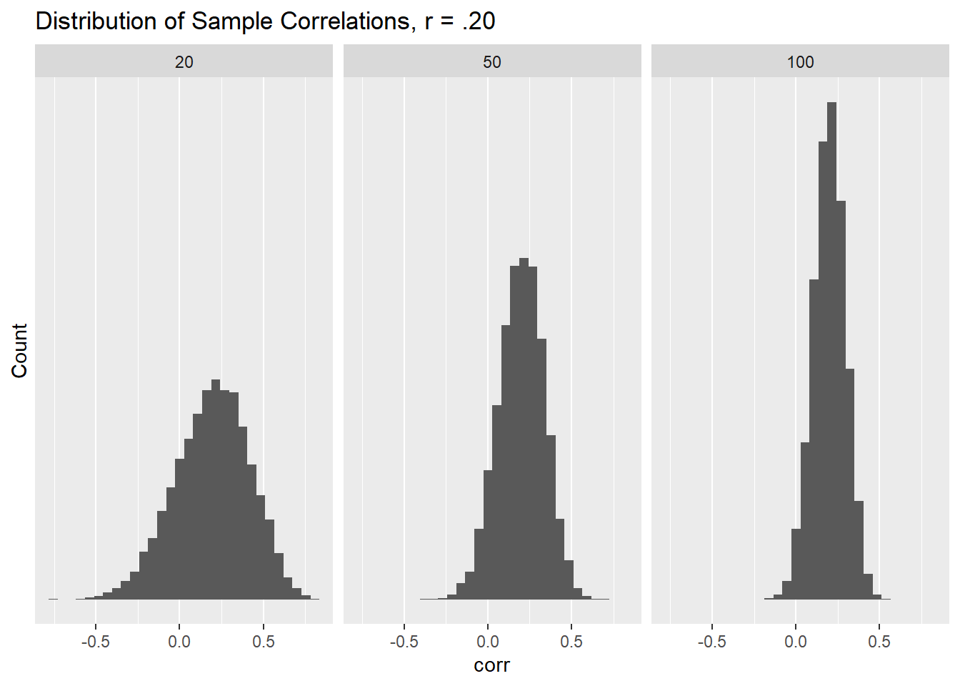
That worked well. I’m not sure precisely what I’m going to do yet for class (whether pass out the above or something different), but it should be straightforward to adapt this to anything else.
The second is to make a line graph for percentage of negative correlations. This is a little trickier.
ggplot(data = perc_neg_corr_final_xy, mapping = aes(x = pop_r, y = perc_neg_xy, group = n, color = factor(n))) +
  geom_point() +
  geom_line() +
  labs(title = "Percent Negative Sample Correlations per Population Correlation and n",
       x = "population correlation", y = "% negative sample correlations", color = "n")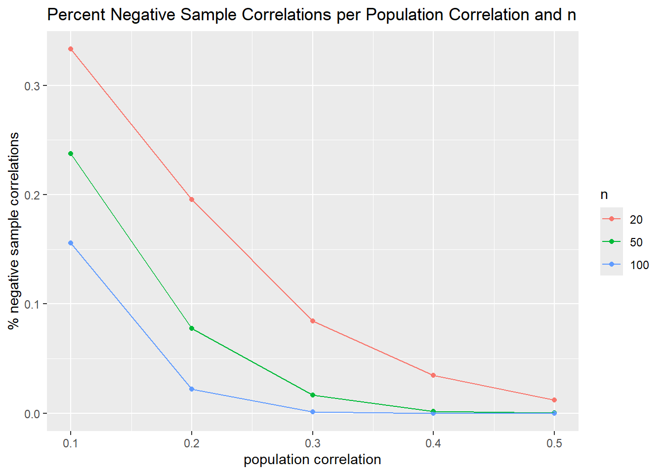
Okay, cool. This worked well.